up:: RDL MOC
lecture07-path-planning-and-obstacle-avoidance-0.pdf
From Grid Maps to Graphs
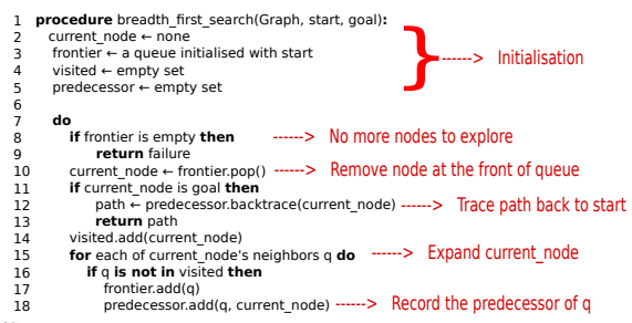
Breadth-First Search
A Brute-force Approach
Given: Graph, start node, goal node.
- Begin search at the start node and do a test for goal.
- If start is same as goal, then stop search.
- Otherwise, continue search.
- Visit the adjacent nodes of start and test whether any of them is goal.
- If goal not found, then continue search at the adjacent nodes of the nodes visited in previous step. Skip any node that has already been visited.
- Continue Step 3, until either the goal is found or until all nodes that can be reached from start node have been visited.
Exhaustive or brute-force search strategy
- Enumerate systematically all possible candidates and test if any of them is the goal.
- In breadth-first search, all paths of length ‘n’ from start are
Inplementaion
Creates and maintains three lists:
- A list of visited nodes. I These nodes have failed the test for goal node.
- A list of frontier nodes. I Frontier nodes are the neighbours of already visited nodes that have not been visited (goal-tested) yet.
- A list of predecessor nodes. I Predecessor is recorded when a node is expanded, i.e. when its neighbours are added to the frontier list.
Pros
- Simple and easy to implement.
- If a path exists from start to goal, it will always find the shortest path (complete and optimal).
- Suitable for smaller grids (fewer cells).
Cons
Link to original
- Searches ‘blindly’. Only adjacency or neighbourhood information is used. (Uninformed search)
- Inefficient, especially for large grids populated sparsely with obstacles.

Informed Search Strategies
Informed Search Strategies
Link to original
- Informed search strategies use knowledge about the problem domain to guide the search more efficiently.
- They evaluate each node using a cost function.
- In path planning problems, the most commonly used cost functions include the estimated distance to the goal node and the actual distance from the start node.
- Informed search strategies are greedy best-first approaches. I Instead of exploring all nodes with equal priority, informed search prioritises the exploration of those nodes that have a lower cost.
Best-First Strategy
A-Star Algorithm
Concept
- Heuristic h(q): Estimated length of the path from the node q to the goal node.
- Exact cost g(q): Length of the actual path from the start node to the node q.
- Total cost for node q: f (q) = h(q) + g(q)
Admissible Heuristic
To find an optimal (least-cost) path from start to goal, the heuristic used by A* should be admissible, i.e. it should never overestimate the actual cost of getting to goal node from the current node.
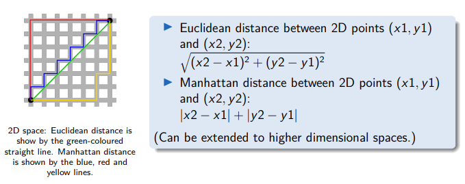
- For a continuous environment (e.g., outdoor feature maps): Euclidean distance, spherical distance, etc.
- For a discrete environment (e.g., indoor occupancy grid maps): Manhattan distance.
Pseudocode
Link to original


Dijkstra’s Algorithm
Allgemein
- Best-First-Search
- Sehr große Graphen – z.B. Routenplaner
- Bei negative Kantengewichte nicht korrekt! → Bellmann-Ford Algorithmus
Definition
Laufzeit
Notizen aus RDL
- However, unlike A*, its cost function has only one term, namely the exact cost g(q). This is the actual cost of moving from the start node to node q.
- If the actual cost of moving from a node to an adjacent node is the identical for all nodes in the graph, then Dijkstra’s algorithm is identical to Breadth-First Search.
⇒ ROS 2 Navigation Stack includes Dijkstra’s and A* path planners.
Link to original


Influence of Grid Map Resolution
Influence of Grid Map Resolution
Link to original

Obstacle Avoidance
Static versus Dynamic Environment
Path planning finds a globally optimal path to reach the goal pose from the initial pose.
However, it assumes a static world, i.e. the positions of obstacles are fixed and fully known. I But, real-world environments are dynamic.
Obstacles may change position dynamically (e.g. furniture may get displaced).
New obstacles may appear on the scene (e.g. something falls down from the overhead shelf).
Obstacles may be constantly moving (e.g. people or other robots moving through corridors).
Global path planning is slow and hence not suitable for fast obstacle avoidance.
Local Approaches
Local Approaches
Basic Idea
- Sensor data (e.g. lidar, sonar) is used to continuously detect obstacles as the robot moves.
- Odometry data is used to obtain the robot’s current pose and velocity.
- A set of possible solutions (candidates) are generated based on sensor and odometry data to steer the robot.
- An objective function evaluates each possible solution.
- The best (optimal) solution is selected and used to control the robot’s linear and angular velocities.
Only a local region around the robot or a short time window is considered at a time for Obstacle Avoidance ⇒ locally optimal motion control.Categories of Approaches
Link to original
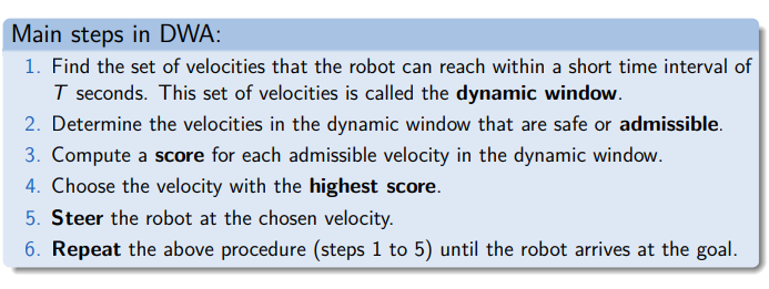
Link to originalDynamic Window Approach
Main Steps
Velocity Space
⇒ Admissible: Grey Area, Non Admissible: Brown Area
⇒ white BoxObjective function F(v, ω)
The objective function F(v, ω) evaluates trajectories based on three criteria:
- Closeness to goal pose: How close to the goal pose would this trajectory bring the robot?
- Clearance from nearest obstacles: How far is the nearest obstacle on this trajectory?
- Speed of motion: How fast does the robot move on this trajectory? I The objective is to drive in the correct direction as fast as possible while staying as far away from obstacles as possible.
Strengths and Weaknesses
Strength:
Fast approach for Obstacle Avoidance.
Weakness:
Difficulty to enter narrow passages and doorways (robot does not stop on time).
Improved DWA:
Optimize position and velocity simultaneously.
Link to original


ROS 2 Navigation Stack
ROS 2 Navigation Stack
Planner Server
Global path planning
A* etcController Server
- Obstical avoidance
Controller Server
- Liniar and Angular Velocity
Behavior Tree
how the robot should react
Link to original
For example: If fails the robot should retry or start recovery strategy

next: RDL VL 08 Task planning